Create trade-off curves

About trade-off curves

A trade-off curve is used to identify optimal materials in designs where there are conflicting objectives (e.g. minimizing both cost and mass) and one limiting constraint (e.g. stiffness-limited design, or strength-limited design). The final material choice is often a compromise.

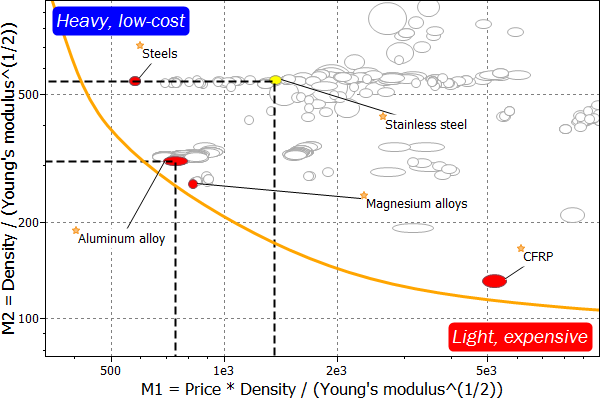
An example trade-off curve for selecting materials for a bicycle is shown below. This is a stiffness-limited design, with two conflicting objectives: to minimize cost, and minimize mass. The free variable is the cross-sectional area.

The performance indices for the two objectives are plotted on the chart axes. For trade-off curves, the convention is to invert the performance indices if necessary so that the objectives are optimized when the indices (M₁ and M₂) are minimized.

Ideal materials that optimize both objectives would be located in the bottom left corner of the chart. As there is no obvious optimum material, a trade-off curve can be used to help visualize which material best matches the objectives.

All materials that lie along the trade-off curve are candidate materials. Materials at the ends of the curve satisfy one of the objectives at the expense of the other. For example, CFRP (carbon fiber reinforced polymer) is low mass but high cost, whereas steel is low cost but high mass. Between the two extremes are materials, such as aluminum and magnesium alloys, that offer a compromise between the two objectives.

The final material choice will depend on the end application, or user of the product, and the relative importance of each objective. For example, a professional racing cyclist would be interested in a bicycle to maximize performance, and would therefore select a composite bicycle in order to minimize mass. Alternatively, a consumer who wants a children’s bicycle would probably opt for a cheaper but ultimately heavier bicycle made from steel.

Create a trade-off curve

To create a trade-off curve:

1. Identify the two conflicting objectives.
   • For the bicycle example above, the two objectives are to minimize mass and to minimize cost, with a stiffness-limited design.
2. Calculate the two performance indices associated with these objectives.
   • Either derive the indices from first principles, use the performance index finder, or consult a table of commonly-used indices .
   • The bicycle frame is modeled as a stiffness-limited beam in bending, with a free sectional area.
     • The performance index to minimize for minimum cost: M₁ = C_m ρ / E^1/2.
     • The performance index to minimize for minimum mass: M₂ = ρ / E^1/2.
     • C_m = material cost per unit mass, ρ = density, E = Young’s modulus (N.B. Flexural modulus can be substituted by Young’s modulus for some materials, and they are assumed here to be the same).
3. Create a chart with M₁ on the x-axis and M₂ on the y-axis.
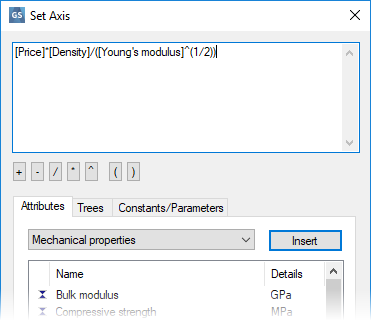
   1. Performance indices can be plotted on a chart axis by building an attribute expression. On the axis tab in the Chart Stage Settings dialog, click Advanced.
   2. Create an expression for the performance index from the list of attributes.
      
4. Create a trade-off curve on the chart.
   1. Click Curve on the chart stage toolbar.
   2. Click on the chart where you want the curve to start.
   3. Click other positions on the chart to create more points.
   4. To finish drawing the curve, press Enter, or double-click on the final point.
5. Drag the curve to adjust the position of it if necessary.

Material selection: graphical method

The trade-off curve is a visual annotation to the chart. All the materials that lie along the trade-off curve are potential candidates, as there are no other materials that have lower values of both M₁ and M₂. These materials are known as non-dominated solutions, and are labelled below in red. The final choice of material will depend on the relative importance of the two objectives.

Materials that lie within the trade-off curve, such as stainless steel, are dominated solutions. These materials are sub-optimal, as there are other materials with lower values of M₁ and/or M₂.

Material selection: penalty functions

About penalty functions

One challenge when using trade-off curves is how to objectively identify which section of the curve contains materials optimal for your application. All materials along the trade-off curve are candidate materials, but which material offers the best balance between minimizing mass and minimizing cost?

The optimum material can be determined by using a penalty function. This is a method that uses exchange constants to determine the relative importance of the conflicting objectives.

The penalty function, Z, is defined as Z = α₁M₁ + α₂M₂ where M₁ and M₂ are the performance indices for the two objectives, and α₁ and α₂ are the exchange constants. Optimum materials are those with the smallest value of Z.

The penalty function is measured in the same units as one of the objectives (often cost). The exchange constants convert the objectives into the same units as Z.

Using the bicycle example, where the objectives are to minimize both mass (M₂) and cost (M₁), Z is set to be measured in units of currency. The exchange constant for the cost is α₁=1, and the units for α₂ are currency/mass. The value of α₂ reflects how much the user is willing to pay for each unit of weight saving, and determines the relative importance of reducing cost over mass.

This allows us to simplify the penalty function to:

Z = α₁ M₁ + α₂ M₂

Z = M₁ + α M₂

Rearranging in terms of the y-axis index (M₂):

M₂ = - M₁/α + Z/α.

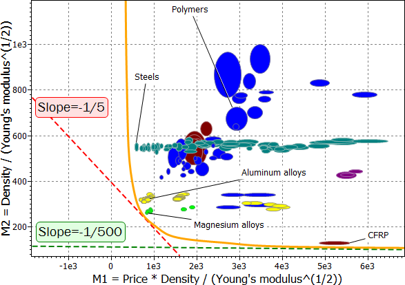
This is an equation for a straight line in the form of y=mx+c. This means we can identify optimal materials by adding a display line of slope -1/α to the trade-off plot with linear scales to find materials that minimize Z. This procedure is detailed below.

Plot a penalty function as a line

To use penalty functions with a trade-off curve chart:

1. Create a trade-off curve on a chart with linear scales.
2. Calculate or look up the value of the exchange constant.
3. Create a display line with slope -1/α.
   1. Click Index and display lines.
   2. Type in the slope value in decimal form.
   3. Select Minimize the index.
   4. Click OK, and then click on the chart to position the line through that point.
4. Move the line so it is tangential to the trade-off curve, and then drag the line upwards until the first set of materials are below the line.
   • The optimal materials are the ones below the penalty function line, close to the trade-off curve.

The chart above is for selecting materials to build a truck, using an exchange constant α=$5/kg (which means that the user/manufacturer is prepared to pay an extra $5 for each kilogram of weight saving). The best materials would be magnesium alloys and aluminum alloys, as these are closest to the display line of low Z (the line tangential to the trade-off curve). Polymers and composites would be least appropriate, as these materials have higher values of Z.

The choice of optimal material for an application will vary depending on the value of the exchange constant. Although magnesium alloys and aluminum alloys are good materials for making a truck, they are not good materials to use for a military aircraft, where saving weight is much more important than minimizing cost. The exchange constant for a military aircraft is α=$500/kg, and optimal materials would be composites like CFRP.

This type of chart allows you to plot lines for different values of exchange constant on the same chart, and to directly compare material choices for different applications.

Plot a penalty function using a combined property

The penalty function can also be evaluated by plotting it as a combined property on a bar chart:

1. Derive an expression for the penalty function.
   • For a stiffness-limited beam in bending, minimizing mass and cost, the penalty function is:

     

     

     

2. Create a new chart stage, and in the Chart Stage Settings dialog, click Advanced on the y-axis tab to create an attribute expression.
3. Enter an expression for the penalty function by adding the required attributes and the value of the exchange constant.
   

Materials that minimize Z are in the bottom right corner of the chart. The value of Z for each material is affected by the exchange constant value.

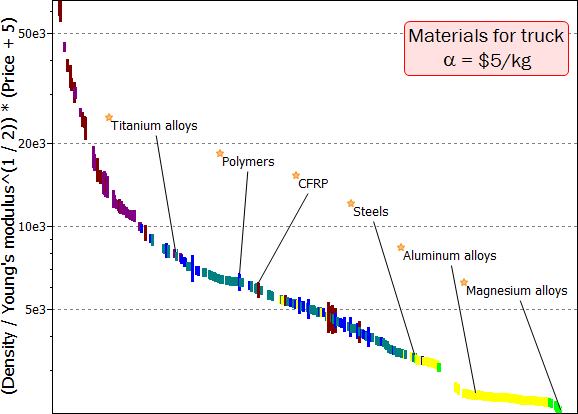
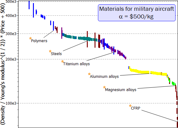
This type of chart makes it easier to evaluate and rank the penalty function for each material. However, it doesn't provide information on which objective has been minimized to produce a low Z value.

Evaluating exchange constants

One of the main challenges in using a penalty function is determining the value of the exchange constant i.e. what the correct balance is between the two conflicting objectives for the design, or, for the bicycle example, how much the user is willing to pay to reduce the bicycle weight. Often this comes down to experience, otherwise it involves significant amounts of research.

For transport vehicles, the exchange constant can be estimated by the fuel cost saving per mass reduction of the vehicle, evaluated over the life of the vehicle. Some of these values are listed below. For other applications, exchange constants can depend on other properties such as performance, style, and perceived worth of a product to a consumer.

Transport vehicle	Basis of estimate	Exchange constant ($/kg)
Family car	Fuel saving	1-2
Truck	Payload	5-20
Civil aircraft	Payload	100-500
Military aircraft	Payload, performance	500-1000
Space vehicle	Payload	3000-10000